If you, like me, have ended up having to implement GPU kernels that fight the existing ecosystem, then you’ve come to the right place. This is my journey learning Triton to implement sparse MMA (Matrix Multiply-Accumulate, not Mixed Martial Arts).
Triton is perfect when your operations vectorize cleanly and don’t need atomic tensor access. It abstracts just enough NVIDIA arcana to not be terrifying, and the syntax feels like numpy with a flamethrower.
I’ll skip the hello-world element-wise ops and jump straight to GEMM (General Matrix Multiplication) for sm8x (Ampere/Ada).
But first, here’s the minimal GPU primer we’ll actually need.
Understanding GPUs
What is sm8x? It’s NVIDIA’s shorthand for GPU generations.
Recent GPUs have: CUDA Cores, Tensor Cores, Global Memory, L2 Cache, Shared Memory, L1 Cache, and Register Memory.
On the software pipeline side, the smallest unit of execution is a thread, which can form a thread group (4 threads), warp (32 threads), and warp groups (4 warps). Yet, the fundamental unit in GPUs is the warp.
Warp-cracy Caste System
Warps are first-class citizens; they are an inseparable clique of 32 homies who must execute the same instruction in lockstep. When one homie diverges and picks a different hobby, the whole crew waits for his return. Several warps form a CTA (Cooperative Thread Array, aka threadblock) to share memory and gossip.
Each thread runs on a CUDA core; when one stalls, the scheduler yeets another thread onto that core to keep it busy.
Tensor Cores are the warps’ personal MMA trainers: specialized hardware for offloading small matrix ops. Each CTA runs on one SM (Streaming Multiprocessor). The RTX 3090 has 82 SMs, and if your CTA is small enough, multiple CTAs can share an SM like roommates.
An NVIDIA GPU has several types of memory, from slowest to fastest:
Global Memory: The VRAM warehouse, 24GB on an RTX 3090.
L2 Cache: 6MB on-die, ~2× faster than global, autopilot with the possibility to skip it.
Shared Memory: ~100KB/SM on an RTX 3090, 10× faster than L2, CTA-exclusive.
L1 Cache: Just read-only shared memory (a.k.a. “Shader Memory” in gaming).
Register Memory: Thread-local, one-cycle access. It doesn’t get faster than this.
GPU Cycle
A GPU cycle is its fundamental time step. For a GPU running at a 2000 MHz clock speed, one cycle takes only 0.5 nanoseconds. Blink, and you’ll miss 2 billion of them.
Memory vs. Computation
The computational power of GPUs far exceeds their memory bandwidth (as of this writing).
Ampere’s 3rd-gen Tensor Cores (TC) can crunch a (16,16) × (16,8) float16 MMA in 8 cycles (more details on Ampere). With 328 Tensor Cores (4 per SM on an RTX 3090), theoretical FP16 throughput hits ~122 TFLOPS. But feeding the beast to get those FLOPS requires ~54 TB/s of bandwidth—a check the VRAM can’t cash, and it is even more difficult with the latest-gen TC.
The trick is to consider the Arithmetic Intensity (AI, the true AI) by leveraging the fact that a (M,K) × (K,N) MMA requires MKN operations but only memory access (if managed properly). Crank M, N, and K large enough, and compute hides memory latency.
Let’s set , with A = 122 TFLOPS and B = 900 GB/s bandwidth. Solve M²×2/B = M³/A → M ≈ 278. Let’s settle for .
Reality check: 122 TFLOPS assumes all 328 Tensor Cores run full-tilt with zero overhead. A 256³ tile needs ~128KB, but bytes/warp/SM limits, copy costs, and K-dimension accumulation add up.
Solution: Each TC handles an m16n8k16 MMA instruction. Make each warp handle one or several m16n8 tiles to avoid the need to accumulate/gather over the k-dimension across warps. For data needed by each warp, we use Shared Memory so that CTA warps can reuse already copied inputs. Then we try to issue as many Tensor Core MMAs as possible while the warps are preparing data (pipelining/multi-staging).
But not all ops are MMA: An element-wise add, for instance, is a memory-bound disaster with 2 reads + 1 write per op = an AI of 1/3. At 900 GB/s, you’re capped at ~300 GFLOPS, the economy class of compute.
Kernel breakdown
Let’s now dive straight into implementing an FP16 GEMM. The matrix has dimensions and matrix has dimensions . Instead of an element-wise implementation, we will use a block-wise approach with tiles of size to match the logic of CUDA programming.
MMA Order
The first thing to consider when implementing Triton kernels is the L2 cache hit rate. For instance, a naive approach might require loading 5 x 8 tiles (8 from A and 32 from B) to compute 4 blocks of C, with all of them being read for the first time from global memory.
(a)Row by row
(b)M-grouped blocks
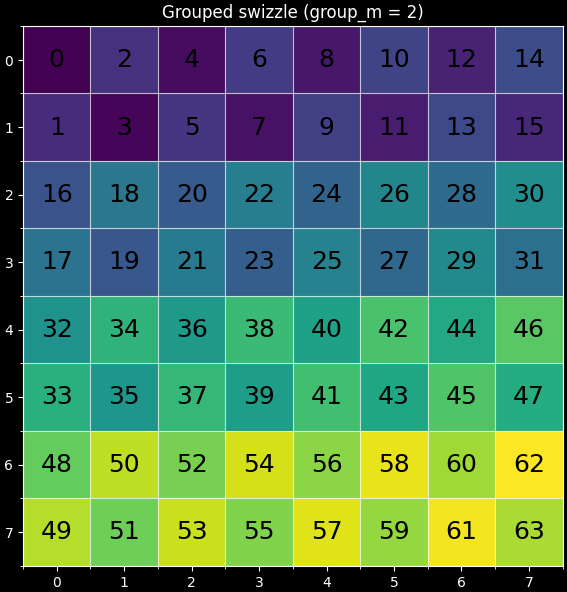
A better approach is to compute a 2x2 tile of blocks of C Figure 1b. This is because when we copy from global memory, the blocks are kept in the L2 cache. A second use of each block-row of A (or block-column of B) will then utilize the cached data, which is roughly twice as fast as accessing global memory. So the first approach will preform 5 row/column reads from global memory, while the second approach only performs 4. According to the tutorial from the Triton documentation, we should expect about a 10% speedup. This will be implemented using a group_m argument, with Figure 2 showing the case for group_m=2.
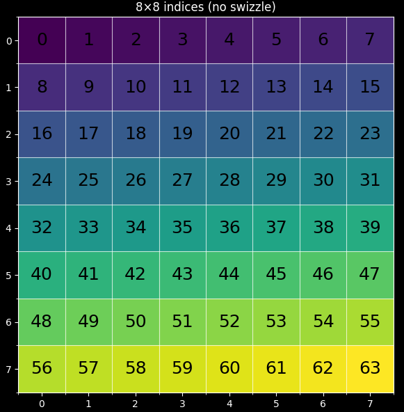
(a)lexical order
(b)Swizzled order
At this stage, we assume we know the memory layout for the matrices: A is row-major, B is column-major, and C is row-major.
row-major
For a row-major matrix of shape , the rows are stored one after the other, so the element is at offset . For a column-major matrix B of shape , the element is at offset .
Triton Syntax
Let’s assume that , and to match the shapes in our examples. We will name our Triton kernel gemm_kernel, which will launch an grid of programs to handle each output tile of .
import triton
import triton.language as tl

@triton.jit
def gemm_kernel(
        a_ptr,
        b_ptr,
        c_ptr,
        m, n, k,
        block_m: tl.constexpr,
        block_n: tl.constexpr,
        block_k: tl.constexpr,
        group_m: tl.constexpr,
        **kwargs
):
    pass
tl.constexpr signifies that these arguments are compile-time constants, and the kernel is recompiled for each new set of these values. It’s customary to use uppercase variables in Triton kernels. However, be aware that the language server might interpret these as global variables, which can lead to unexpected errors if they are modified outside their intended scope.
Since each kernel call handles one tile of C, how does it know which tile to process? The answer is not very Pythonic; we use tl.program_id within the kernel’s scope:
pid_m = tl.program_id(axis=0)
pid_n = tl.program_id(axis=1)
We must then ensure the kernel is launched with the correct grid dimensions (for our specific case):
gemm_kernel[(8, 4)](arguments...)Instead of a fixed grid like (8,4), we can also use a function that takes the arguments of gemm_kernel and returns the grid size dynamically.
Let’s assume the kernel is implemented. We can run it as follows:
import torch

def matmul(a: torch.Tensor, b: torch.Tensor, block_m=128, block_n=128, block_k=64, group_m=8):
    m, k = a.shape
    k_b, n = b.shape
    assert k == k_b
    assert b.stride(0) == 1 # b is column major

    c = torch.empty((m, n), device=a.device, dtype=a.dtype)

    grid = (triton.cdiv(m, block_m), triton.cdiv(n, block_n))
    gemm_kernel[grid](
        a,
        b,
        c,
        m,
        n,
        k,
        block_m,
        block_n,
        block_k,
        group_m
    )
    return c
GEMM Kernel
The next step is to loop over the K dimension and:
Copy blocks of A and B.
Multiply and accumulate the results.
Store the final result.
All these steps require defining the correct offsets from which we read and to which we write.
For instance, for the first block of A (where pid_m=0, pid_n=0), we need the following indices:
A_offsets = [[0, 1, 2, ..., block_k-1],
             [K, K+1, ..., K + block_k-1],
             ...
             [(block_m-1) * K, ..., (block_m-1) * K + block_k-1]]
So that A_ptr+A_offsets is a (block_m, block_k) pointer. Similar logic applies to other operations.
Now let’s define the base indices that we will offset as we iterate through the blocks:
offs_am = pid_m * block_m + tl.arange(0, block_m)
offs_bn = pid_n * block_n + tl.arange(0, block_n)
offs_k = tl.arange(0, block_k)
And define our vectorized pointers as:
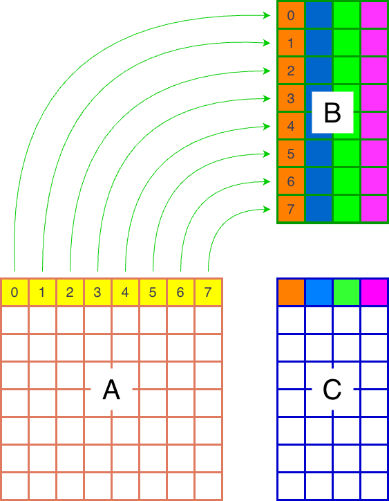
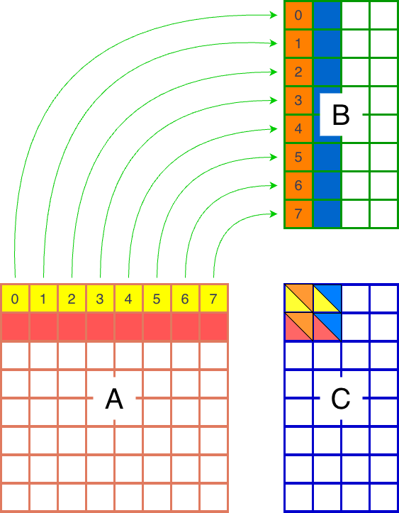
a_ptrs = a_ptr + offs_am[:, None] * K + offs_k[None, :] # A is row-major
b_ptrs = b_ptr + offs_k[:, None] + offs_bn[None, :] * K # B is column-major
To move the pointer to the next block, we simply increment it by block_k for A and B.
Visualizing indices
You can use numpy to see what the indices are:
import numpy as np


K = 512

pid_m = 0
pid_n = 0
block_m = 16
block_n = 16
block_k = 32

offs_am = pid_m * block_m + np.arange(0, block_m)
offs_bn = pid_n * block_n + np.arange(0, block_n)
offs_k = np.arange(0, block_k)
print("A offsets", offs_am[:, None] * K + offs_k[None, :] )
print("B offsets", offs_k[:, None] + offs_bn[None, :] * K)
Let’s now initialize our accumulator:
accumulator = tl.zeros((block_m, block_n), dtype=tl.float32)And start the MMA loop:
for k_loop in range(0, tl.cdiv(k, block_k)):

    k_remaining = k - k_loop * block_k # used for boundary check
    mask = offs_k < k_remaining

    a = tl.load(a_ptrs, mask=mask[None, :], other=0.0)
    b = tl.load(b_ptrs, mask=mask[:, None], other=0.0)

    accumulator = tl.dot(a, b, accumulator)
    a_ptrs += block_k
    b_ptrs += block_k
When we load blocks of A and B, we must ensure that we do not go out of the bounds of the K dimension. This is usually not an issue when is a multiple of (common in neural networks), but it is generally not the case. The masking approach handles these boundary conditions cleanly. The other=0.0 argument ensures that out-of-bounds elements are loaded as zero, preventing them from affecting the computation. The mask expression is equivalent to:
mask = offs_k + k_loop * block_k < k - k_remainingbut the hack above avoids materializing the vector offs_k + k_loop * block_k (I don’t know if it improves performance, TODO).
The final step is to store the accumulator block:
# convert accumulator to the target c type
c = accumulator.to(c_ptr.dtype.element_ty)

# create the offsets
offs_cm = pid_m * block_m + tl.arange(0, block_m)
offs_cn = pid_n * block_n + tl.arange(0, block_n)
c_ptrs = c_ptr + offs_cm[:, None] * n + offs_cn[None, :]
c_mask = (offs_cm[:, None] < m) & (offs_cn[None, :] < n)
tl.store(c_ptrs, c, mask=c_mask)
Kernel Finetuning
The next step is to find the optimal values for:
block_m,block_n,block_k,group_mnum_warps: the number of warp threads involved in the program.num_stages: how many tiles of A and B are being copied while the GPU computes the MMA for other blocks. This is also known as pipelining.
num_warps and num_stages are arguments to the kernel launch. num_warps is expected to be a power of 2. num_stages determines how many for loop iterations get their tl.load calls unrolled so that when the loop computation is handled, the data blocks are already in shared memory. If num_stages requires more shared memory than is available, Triton will throw an error.
To find the best parameters, Triton has a built-in feature to perform a parameter sweep for each combination of key values (m,n,k combo),
by decorating the kernel
import triton

@triton.autotune(
    configs=[
        triton.Config({'block_m': 128, 'block_n': 256, 'block_k': 64, 'group_m': 8}, num_stages=3, num_warps=8),
        triton.Config({'block_m': 64, 'block_n': 256, 'block_k': 32, 'group_m': 8}, num_stages=4, num_warps=4),
        triton.Config({'block_m': 128, 'block_n': 128, 'block_k': 32, 'group_m': 8}, num_stages=4, num_warps=4),
        triton.Config({'block_m': 128, 'block_n': 64, 'block_k': 32, 'group_m': 8}, num_stages=4, num_warps=4),
        triton.Config({'block_m': 64, 'block_n': 128, 'block_k': 32, 'group_m': 8}, num_stages=4, num_warps=4),
        triton.Config({'block_m': 128, 'block_n': 32, 'block_k': 32, 'group_m': 8}, num_stages=4, num_warps=4),
        triton.Config({'block_m': 64, 'block_n': 32, 'block_k': 32, 'group_m': 8}, num_stages=5, num_warps=2),
        triton.Config({'block_m': 32, 'block_n': 64, 'block_k': 32, 'group_m': 8}, num_stages=5, num_warps=2),
    ],
    key=['m', 'n', 'k']
)
@triton.jit
def gemm_kernel(......):
    # ... kernel implementation
    pass
This can be a laborious process, but it is suitable when we have a clear idea of what the kernel does and what the best values could be.
Cooking
Let’s put everything together now to run our gemm kernel.
I’ll be using a more generic kernel that handles all layouts for A, B, and C instead of assuming they’re row/column major.
The version bellow takes into account all types of layout combos for A,B,C. For instance, a row major A would have strides
stride_am, stride_ak=(k,1) while a col-major would use (1,m).
import triton
import triton.language as tl


@triton.jit
def matmul_kernel(
    a_ptr,
    b_ptr,
    c_ptr,
    m,
    n,
    k,
    stride_am,
    stride_ak,
    stride_bk,
    stride_bn,
    stride_cm,
    stride_cn,
    block_m: tl.constexpr,
    block_n: tl.constexpr,
    block_k: tl.constexpr,
    group_m: tl.constexpr,
):
    """Kernel for computing the matmul C = A x B.
    A has shape (M, K), B has shape (K, N) and C has shape (M, N)
    """
    pid_m = tl.program_id(axis=0)
    pid_n = tl.program_id(axis=1)

    num_pid_m = tl.cdiv(m, block_m)
    num_pid_n = tl.cdiv(n, block_n)

    pid_m, pid_n = tl.swizzle2d(pid_m, pid_n, num_pid_m, num_pid_n, group_m)

    # for compiler
    tl.assume(pid_m >= 0)
    tl.assume(pid_n >= 0)
    tl.assume(stride_am > 0)
    tl.assume(stride_ak > 0)
    tl.assume(stride_bn > 0)
    tl.assume(stride_bk > 0)
    tl.assume(stride_cm > 0)
    tl.assume(stride_cn > 0)
    # ----------------------
    offs_am = pid_m * block_m + tl.arange(0, block_m)
    offs_bn = pid_n * block_n + tl.arange(0, block_n)
    offs_k = tl.arange(0, block_k)

    a_ptrs = a_ptr + (
        offs_am[:, None] * stride_am + offs_k[None, :] * stride_ak
    )

    b_ptrs = b_ptr + (
        offs_k[:, None] * stride_bk + offs_bn[None, :] * stride_bn
    )

    accumulator = tl.zeros((block_m, block_n), dtype=tl.float32)
    for k_loop in range(0, tl.cdiv(k, block_k)):
        k_remaining = k - k_loop * block_k

        mask = offs_k < k_remaining
        a = tl.load(a_ptrs, mask=mask[None, :], other=0.0)
        b = tl.load(b_ptrs, mask=mask[:, None], other=0.0)

        accumulator = tl.dot(a, b, accumulator)
        a_ptrs += block_k * stride_ak
        b_ptrs += block_k * stride_bk

    c = accumulator.to(c_ptr.dtype.element_ty)

    offs_cm = pid_m * block_m + tl.arange(0, block_m)
    offs_cn = pid_n * block_n + tl.arange(0, block_n)
    c_ptrs = c_ptr + stride_cm * offs_cm[:, None] + stride_cn * offs_cn[None, :]
    c_mask = (offs_cm[:, None] < m) & (offs_cn[None, :] < n)
    tl.store(c_ptrs, c, mask=c_mask)
Kernel Fine-tuning
When implementing Triton kernels, I prefer to structure my packages so that the raw kernels reside in a separate module.
To avoid cluttering the kernel definition with hardcoded autotune decorators, I use a specific wrapper pattern.
While there are (standard) approaches from Triton docs such as filtering configurations via a prune_configs_by argument, I find them somewhat invasive.
For reference, the pruning approach from Triton docs looks like this:
def prune_invalid_configs(configs, named_args, **kwargs):
    m, n, k = named_args["m"], named_args["n"], named_args["k"]
    # ... filter out configs based on m, n, k
    return pruned_configs

# Usage in the decorator
@triton.autotune(configs=configs, key=["m", "n", "k"],
                 prune_configs_by={'early_config_prune': prune_invalid_configs})
def matmul_kernel(...): ...
My preferred approach decouples the autotuning logic from the kernel definition:
# 1. Define specialization keys as an attribute of the raw kernel
matmul_kernel.specialize_keys = ["m", "n", "k"]

# 2. Use a helper to apply the autotuner dynamically
def wrap_autotuner(kernel, configs, reset_to_zero=None, restore_value=None):
    """
    Wraps a Triton kernel with autotuning capabilities.
    """
    return Autotuner(
        kernel,
        kernel.arg_names,
        configs=configs,
        key=kernel.specialize_keys,
        reset_to_zero=reset_to_zero,
        restore_value=restore_value,
    )
We can then generate configurations using a helper function (e.g., get_autotune_configs) and run the benchmark:
import statistics
import torch
import triton

SHAPES = [
    (256, 256, 256),
    (512, 512, 512),
    (1024, 1024, 1024),
    (2048, 2048, 2048),
    (4096, 4096, 4096),
]

DTYPE = torch.float16
WARMUP = 10
ITERS = 50

def tflops(m: int, n: int, k: int, mean_ms: float) -> float:
    return (2.0 * m * n * k) / (mean_ms * 1e9)

def time_loop_ms(fn, *, warmup: int, iters: int) -> tuple[float, float, float]:
    for _ in range(warmup):
        fn()
    torch.cuda.synchronize()
    lapses = []

    for _ in range(iters):
        start = torch.cuda.Event(enable_timing=True)
        end = torch.cuda.Event(enable_timing=True)
        start.record()
        fn()
        end.record()
        torch.cuda.synchronize()
        lapses.append(start.elapsed_time(end))
    return (
        statistics.fmean(lapses),
        statistics.median(lapses),
        statistics.pstdev(lapses),
    )

def main() -> None:
    torch.manual_seed(0)
    torch.cuda.manual_seed(0)

    device = torch.device("cuda")
    props = torch.cuda.get_device_properties(device)
    print(f"Device: {props.name} (SM {props.major}{props.minor}), dtype={DTYPE}")
    print(f"Warmup/iters: {WARMUP}/{ITERS}")

    configs = get_autotune_configs()
    tuned = wrap_autotuner(matmul_kernel, configs)

    print(
        "M      N      K | best_config                 |  triton_ms  triton_TF |   torch_ms   torch_TF | speedup"
    )
    print("-" * 110)

    for m, n, k in SHAPES:
        a = torch.randn((m, k), device=device, dtype=DTYPE).contiguous()
        b = torch.randn((k, n), device=device, dtype=DTYPE).contiguous()
        out_triton = torch.empty((m, n), device=device, dtype=DTYPE)
        out_torch = torch.empty((m, n), device=device, dtype=DTYPE)

        def grid(meta):
            return (
                triton.cdiv(m, meta["block_m"]),
                triton.cdiv(n, meta["block_n"]),
            )

        # Compile + autotune once per shape.
        tuned[grid](
            a, b, out_triton, m, n, k,
            a.stride(0), a.stride(1),
            b.stride(0), b.stride(1),
            out_triton.stride(0), out_triton.stride(1),
        )
        torch.cuda.synchronize()

        # Retrieve best config from cache
        cache_key = (m, n, k, str(a.dtype), str(b.dtype), str(out_triton.dtype))
        best = tuned.cache.get(cache_key)

        if best is None:
            best_str = "(missing)"
        else:
            kw = best.kwargs
            best_str = (
                f"{kw['block_m']}x{kw['block_n']}x{kw['block_k']} "
                f"gm{kw['group_m']} w{best.num_warps} s{best.num_stages}"
            )

        def run_triton() -> None:
            tuned[grid](
                a, b, out_triton, m, n, k,
                a.stride(0), a.stride(1),
                b.stride(0), b.stride(1),
                out_triton.stride(0), out_triton.stride(1),
            )

        def run_torch() -> None:
            torch.matmul(a, b, out=out_torch)

        tr_mean, _, _ = time_loop_ms(run_triton, warmup=WARMUP, iters=ITERS)
        th_mean, _, _ = time_loop_ms(run_torch, warmup=WARMUP, iters=ITERS)

        tr_tf = tflops(m, n, k, tr_mean)
        th_tf = tflops(m, n, k, th_mean)
        speedup = th_mean / tr_mean if tr_mean > 0 else float("inf")

        print(
            f"{m:6d} {n:6d} {k:6d} | "
            f"{best_str:<22s} | "
            f"{tr_mean:10.3f} {tr_tf:10.2f} | "
            f"{th_mean:10.3f} {th_tf:10.2f} | "
            f"{speedup:5.2f}x"
        )

if __name__ == "__main__":
    main()
This yields the following results:
Device: NVIDIA GeForce RTX 3090 (SM 86), dtype=torch.float16
Warmup/iters: 10/50
M      N      K | best_config                 |  triton_ms  triton_TF |   torch_ms   torch_TF | speedup
-------------------------------------------------------------------------------------------------------------
   256    256    256 | 64x32x32 gm8 w4 s4     |      0.042       0.79 |      0.016       2.07 |  0.38x
   512    512    512 | 128x32x32 gm8 w4 s4    |      0.043       6.29 |      0.016      16.54 |  0.38x
  1024   1024   1024 | 64x64x32 gm8 w4 s4     |      0.077      27.88 |      0.049      44.07 |  0.63x
  2048   2048   2048 | 64x64x32 gm8 w4 s4     |      0.271      63.47 |      0.274      62.76 |  1.01x
  4096   4096   4096 | 128x128x32 gm8 w4 s4   |      1.974      69.61 |      2.017      68.16 |  1.02x

gm: group_m
w: warps
s: stages
For large shapes, we are achieving performance comparable to cuBLAS. However, for smaller shapes, there is still significant room for optimization.